

GRE Prep Club Daily Prep
Thank you for using the timer - this advanced tool can estimate your performance and suggest more practice questions. We have subscribed you to Daily Prep Questions via email.
Customized
for You
Track
Your Progress
Practice
Pays
Not interested in getting valuable practice questions and articles delivered to your email? No problem, unsubscribe here.
 Nov 17
Live Online Classes with Top GRE Expert Rich Zwelling
08:00 PM EST
-10:00 PM EST
Get live instruction from a top-scoring, industry-recognized GRE teachers + 6 months of access to TTP Self-Study included! Tues/Thur Sept 7, 2026---Feb. 2, 2027, 1:00pm-3:00pm EST Dec 14
Live Online Classes with Top GRE Expert Michael Butville
08:00 PM EST
-10:00 PM EST
Get live instruction from a top-scoring, industry-recognized GRE teachers + 6 months of access to TTP Self-Study included! Mon/Wed Dec. 14, 2026---Feb. 22, 2027, 8:00pm-10:00pm EST

GRE Math Essentials The Normal Distribution (Bell Curve)
[#permalink]
 23 Oct 2026, 23:28
Expert Reply
GRE Math Essentials – The Normal Distribution (Bell Curve)
This is part of our GRE Math Essentials - A most comprehensive handout!! — DATA ANALYSIS › SET & STATISTIC Theory.
Before reading this chapter, make sure you are comfortable with Mean, Median, Range, Mode & Standard Deviation.
What you will learn
━━━━━━━━━━━━━━━━━━━━━━━━━━━━━━━━━━━━━━━━
1. What is a normal distribution?
A normal distribution (also called a Gaussian distribution or bell curve) describes data that cluster around a central value and become rarer the farther you move away from it. Heights of adults, measurement errors and scores on large standardized tests are classic examples.
Think of the curve as a "pile" of all the data. The height of the curve shows how common a value is; the area under the curve between two points shows what fraction of the data lies between them. The total area under the whole curve is 100%.
Key properties (memorize these)
Effect of the standard deviation — a small SD gives a tall, narrow curve (data packed near the mean); a large SD gives a short, wide curve (data spread out). The mean only slides the curve left or right.
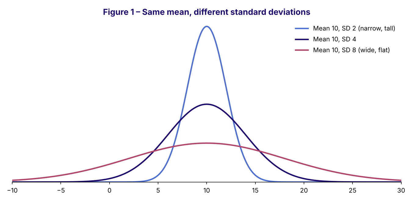
fig1_different_sd.png [ 80.49 KiB | Viewed 52 times ]
━━━━━━━━━━━━━━━━━━━━━━━━━━━━━━━━━━━━━━━━
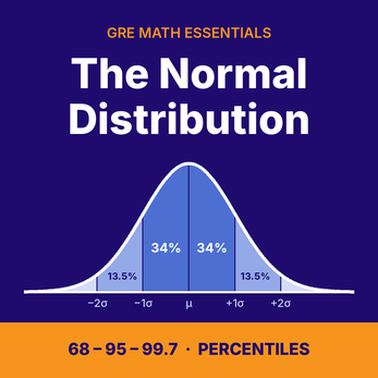
2. The Empirical Rule (68 – 95 – 99.7)
For any normal distribution — whatever its mean and SD — the same fixed percentages of data fall within 1, 2 and 3 standard deviations of the mean:
Note: some prep books round these to "2/3" and "96%". You will get the same answer choices on the GRE with either version — the test always says "approximately" and gives answer choices far enough apart.
The building blocks: split by symmetry
The real power of the rule comes from cutting each band in half, because the curve is symmetric. Going outward from the mean, each side contains:
Check: 34 + 13.5 + 2.35 + 0.15 = 50% on each side. ✔
Example used throughout this chapter: a normal distribution with mean = 10 and SD = 4. Each step of one SD is 4 units, so the marks on the axis are:
-2 (−3σ), 2 (−2σ), 6 (−1σ), 10 (mean), 14 (+1σ), 18 (+2σ), 22 (+3σ).
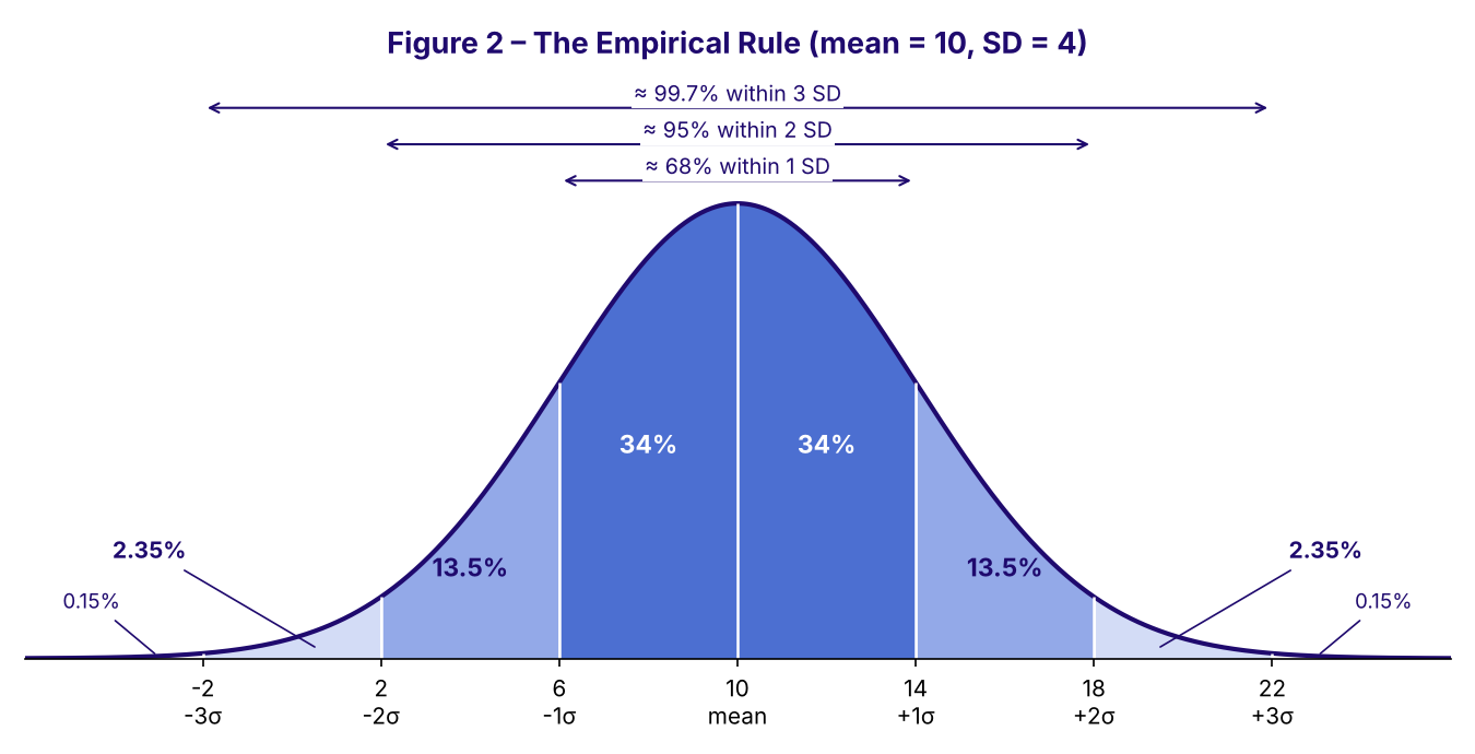
fig2_empirical_rule.png [ 83.2 KiB | Viewed 52 times ]
━━━━━━━━━━━━━━━━━━━━━━━━━━━━━━━━━━━━━━━━
3. From a value to its percentile — the core skill
Definition. The percentile of a value = the percentage of the data that lies below (to the left of) that value. On the bell curve, it is the area to the left.
The 3-step method
Example A – the value 6
(6 − 10) ÷ 4 = −1 → 6 is 1 SD below the mean.
Start at 50%. Moving left from 10 to 6 you cross the 34% slice → 50% − 34% = 16%.
So 6 is at about the 16th percentile: roughly 16% of the data are smaller than 6.
Example B – the value 14
(14 − 10) ÷ 4 = +1 → 1 SD above the mean.
50% + 34% = 84% → about the 84th percentile.
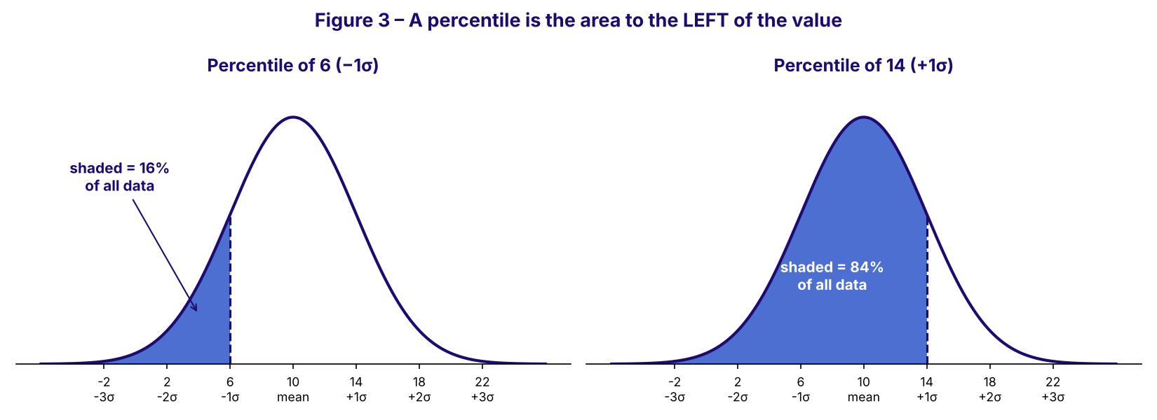
fig3_percentiles.png [ 91.12 KiB | Viewed 51 times ]
Example C – the values 2 and 18
2 is 2 SD below: 50% − 34% − 13.5% = 2.5% → about the 2nd–3rd percentile.
18 is 2 SD above: 50% + 34% + 13.5% = 97.5% → about the 97th–98th percentile.
Why some books write "50% − 1⁄2·(2/3) = 17%" or "50% − 1⁄2·(96%) = 2%"
It is exactly the same idea. "1⁄2 × (share within k SD)" is just one side of the band — the slice between the mean and the value. With the "2/3" rounding, one side is 1/3 ≈ 33%, giving 50 − 33 ≈ 17%; with the "68%" version, one side is 34%, giving 16%. Same logic, slightly different rounding.
Percentile cheat sheet (memorize)
Shortcut: the percentiles on the right side are 100 minus the ones on the left (84 = 100 − 16; 97.5 = 100 − 2.5). That is symmetry at work.
━━━━━━━━━━━━━━━━━━━━━━━━━━━━━━━━━━━━━━━━
4. Percentage of data BETWEEN two values
Just add the slices between the two values.
Example: What percent of the data lies between 6 and 18?
6 is −1σ, 18 is +2σ. The slices between them: 34% (6→10) + 34% (10→14) + 13.5% (14→18) = 81.5%.
Alternative way (percentile difference): percentile(18) − percentile(6) = 97.5% − 16% = 81.5%. ✔
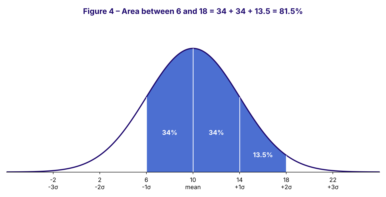
fig4_area_between.png [ 59.19 KiB | Viewed 52 times ]
Above a value = 100% − percentile. E.g. % of data above 14 = 100% − 84% = 16%.
Counting people. If the data describe 2,000 people, the number between 6 and 18 is 81.5% × 2,000 = 1,630. The GRE often hides the percentage inside a "how many" question.
━━━━━━━━━━━━━━━━━━━━━━━━━━━━━━━━━━━━━━━━
5. Working backward: from percentiles to mean and SD
The GRE likes to give you percentiles and ask for the mean or SD. Translate each percentile into an SD position first:
Example: In a normal distribution, the 16th percentile is 38 and the 84th percentile is 62. Find the mean and SD.
The mean is exactly halfway (symmetry): (38 + 62) ÷ 2 = 50.
From 50 to 62 is 1 SD → SD = 12.
━━━━━━━━━━━━━━━━━━━━━━━━━━━━━━━━━━━━━━━━
6. Comparing values from different distributions
A raw score means little on its own; what matters is how many SDs it is from its own mean (this number is called a z-score, z = (value − mean) ÷ SD).
Example: Ana scores 85 on a test with mean 70 and SD 10. Ben scores 90 on a test with mean 70 and SD 20. Who did better relative to the other test-takers?
Ana: (85 − 70) ÷ 10 = +1.5 SD. Ben: (90 − 70) ÷ 20 = +1 SD.
Ana is farther above her mean → higher percentile, even though Ben's raw score is higher.
━━━━━━━━━━━━━━━━━━━━━━━━━━━━━━━━━━━━━━━━
7. GRE traps to watch for
━━━━━━━━━━━━━━━━━━━━━━━━━━━━━━━━━━━━━━━━
8. Practice questions
Q1. The scores on an exam are normally distributed with a mean of 500 and a standard deviation of 100. Approximately what percentile is a score of 700?
(A) 68th (B) 84th (C) 95th (D) 98th (E) 99.9th
Q2. The heights of a group of adults are normally distributed with a mean of 170 cm and a standard deviation of 6 cm. Approximately what percent of the adults are between 164 cm and 182 cm tall?
(A) 47.5% (B) 68% (C) 81.5% (D) 84% (E) 95%
Q3. A data set is normally distributed with a mean of 40 and a standard deviation of 5.
Quantity A: The percent of the data greater than 50
Quantity B: The percent of the data less than 35
(A) A greater (B) B greater (C) Equal (D) Cannot be determined
Q4. In a normal distribution, the value at the 16th percentile is 38 and the value at the 84th percentile is 62. Approximately which value is at the 2.5th percentile?
(A) 14 (B) 26 (C) 32 (D) 36 (E) 44
Q5. The weights of 1,000 packages are normally distributed. Approximately how many packages weigh between 2 standard deviations below the mean and 1 standard deviation above the mean?
(A) 475 (B) 680 (C) 815 (D) 840 (E) 950
Q6. Carla scored 78 on Test 1 (mean 60, SD 12). Dan scored 88 on Test 2 (mean 64, SD 16). Both sets of scores are normally distributed.
Quantity A: Carla's percentile on Test 1
Quantity B: Dan's percentile on Test 2
(A) A greater (B) B greater (C) Equal (D) Cannot be determined
Q7. A list of numbers has a mean of 20 and a standard deviation of 3.
Quantity A: The percent of the numbers between 17 and 23
Quantity B: 68%
(A) A greater (B) B greater (C) Equal (D) Cannot be determined
Q1 – (D). (700 − 500) ÷ 100 = +2 SD. 50% + 34% + 13.5% = 97.5% ≈ 98th percentile.
Q2 – (C). 164 = 170 − 6 (−1σ); 182 = 170 + 12 (+2σ). 34% + 34% + 13.5% = 81.5%.
Q3 – (B). 50 is +2σ → percent above = 100% − 97.5% = 2.5%. 35 is −1σ → percent below = 16%. B is larger.
Q4 – (B). Mean = (38 + 62) ÷ 2 = 50; SD = 62 − 50 = 12. The 2.5th percentile is mean − 2σ = 50 − 24 = 26.
Q5 – (C). Slices from −2σ to +1σ: 13.5% + 34% + 34% = 81.5%. 81.5% of 1,000 ≈ 815.
Q6 – (C). Carla: (78 − 60) ÷ 12 = +1.5 SD. Dan: (88 − 64) ÷ 16 = +1.5 SD. Same distance in SDs → same percentile, even though the raw scores differ.
Q7 – (D). The list is not stated to be normal. The 68% rule cannot be applied; the percent within 1 SD could be more or less than 68%. Classic trap.
━━━━━━━━━━━━━━━━━━━━━━━━━━━━━━━━━━━━━━━━
Summary in one box
normal_distribution_cover_347.png [ 38.41 KiB | Viewed 58 times ]
This is part of our GRE Math Essentials - A most comprehensive handout!! — DATA ANALYSIS › SET & STATISTIC Theory.
Before reading this chapter, make sure you are comfortable with Mean, Median, Range, Mode & Standard Deviation.
What you will learn
- What a normal distribution is and its key properties
- The Empirical Rule (68 – 95 – 99.7) and the "34 – 13.5 – 2.35" building blocks
- How to turn any value into a percentile (the step most students get stuck on)
- How to find the percentage of data between two values
- How to work backward from percentiles to the mean and standard deviation
- How to compare values from two different distributions
- The traps the GRE sets — and 7 practice questions with solutions
━━━━━━━━━━━━━━━━━━━━━━━━━━━━━━━━━━━━━━━━
1. What is a normal distribution?
A normal distribution (also called a Gaussian distribution or bell curve) describes data that cluster around a central value and become rarer the farther you move away from it. Heights of adults, measurement errors and scores on large standardized tests are classic examples.
Think of the curve as a "pile" of all the data. The height of the curve shows how common a value is; the area under the curve between two points shows what fraction of the data lies between them. The total area under the whole curve is 100%.
Key properties (memorize these)
- Symmetric about the center: the left half is a mirror image of the right half.
- Mean = Median = Mode, all at the center (the peak).
- Because of symmetry, 50% of the data lies below the mean and 50% above it. So the mean is always the 50th percentile.
- The curve is completely determined by two numbers: the mean (where the center is) and the standard deviation, SD or σ (how spread out the data are).
- The tails extend forever in both directions but get very thin very quickly.
Effect of the standard deviation — a small SD gives a tall, narrow curve (data packed near the mean); a large SD gives a short, wide curve (data spread out). The mean only slides the curve left or right.
Attachment:
fig1_different_sd.png [ 80.49 KiB | Viewed 52 times ]
━━━━━━━━━━━━━━━━━━━━━━━━━━━━━━━━━━━━━━━━
2. The Empirical Rule (68 – 95 – 99.7)
For any normal distribution — whatever its mean and SD — the same fixed percentages of data fall within 1, 2 and 3 standard deviations of the mean:
| Range | Share of the data |
| Within 1 SD of the mean (mean ± 1σ) | ≈ 68% (about 2/3) |
| Within 2 SD of the mean (mean ± 2σ) | ≈ 95% |
| Within 3 SD of the mean (mean ± 3σ) | ≈ 99.7% (almost everything) |
Note: some prep books round these to "2/3" and "96%". You will get the same answer choices on the GRE with either version — the test always says "approximately" and gives answer choices far enough apart.
The building blocks: split by symmetry
The real power of the rule comes from cutting each band in half, because the curve is symmetric. Going outward from the mean, each side contains:
| Slice (one side only) | Area |
| mean → 1σ | 34% (half of 68%) |
| 1σ → 2σ | 13.5% (half of 95% − 68% = half of 27%) |
| 2σ → 3σ | 2.35% (half of 99.7% − 95% = half of 4.7%) |
| beyond 3σ | 0.15% (half of 100% − 99.7% = half of 0.3%) |
Check: 34 + 13.5 + 2.35 + 0.15 = 50% on each side. ✔
Example used throughout this chapter: a normal distribution with mean = 10 and SD = 4. Each step of one SD is 4 units, so the marks on the axis are:
-2 (−3σ), 2 (−2σ), 6 (−1σ), 10 (mean), 14 (+1σ), 18 (+2σ), 22 (+3σ).
Attachment:
fig2_empirical_rule.png [ 83.2 KiB | Viewed 52 times ]
━━━━━━━━━━━━━━━━━━━━━━━━━━━━━━━━━━━━━━━━
3. From a value to its percentile — the core skill
Definition. The percentile of a value = the percentage of the data that lies below (to the left of) that value. On the bell curve, it is the area to the left.
The 3-step method
- Locate the value: how many SDs is it above or below the mean?
number of SDs = (value − mean) ÷ SD - Start at the mean, which is always the 50th percentile.
- Add the slices you cross if you move right; subtract them if you move left.
Example A – the value 6
(6 − 10) ÷ 4 = −1 → 6 is 1 SD below the mean.
Start at 50%. Moving left from 10 to 6 you cross the 34% slice → 50% − 34% = 16%.
So 6 is at about the 16th percentile: roughly 16% of the data are smaller than 6.
Example B – the value 14
(14 − 10) ÷ 4 = +1 → 1 SD above the mean.
50% + 34% = 84% → about the 84th percentile.
Attachment:
fig3_percentiles.png [ 91.12 KiB | Viewed 51 times ]
Example C – the values 2 and 18
2 is 2 SD below: 50% − 34% − 13.5% = 2.5% → about the 2nd–3rd percentile.
18 is 2 SD above: 50% + 34% + 13.5% = 97.5% → about the 97th–98th percentile.
Why some books write "50% − 1⁄2·(2/3) = 17%" or "50% − 1⁄2·(96%) = 2%"
It is exactly the same idea. "1⁄2 × (share within k SD)" is just one side of the band — the slice between the mean and the value. With the "2/3" rounding, one side is 1/3 ≈ 33%, giving 50 − 33 ≈ 17%; with the "68%" version, one side is 34%, giving 16%. Same logic, slightly different rounding.
Percentile cheat sheet (memorize)
| Position | −3σ | −2σ | −1σ | mean | +1σ | +2σ | +3σ |
| Value (mean 10, SD 4) | −2 | 2 | 6 | 10 | 14 | 18 | 22 |
| Percentile | ≈ 0.15 | ≈ 2.5 | ≈ 16 | 50 | ≈ 84 | ≈ 97.5 | ≈ 99.85 |
Shortcut: the percentiles on the right side are 100 minus the ones on the left (84 = 100 − 16; 97.5 = 100 − 2.5). That is symmetry at work.
━━━━━━━━━━━━━━━━━━━━━━━━━━━━━━━━━━━━━━━━
4. Percentage of data BETWEEN two values
Just add the slices between the two values.
Example: What percent of the data lies between 6 and 18?
6 is −1σ, 18 is +2σ. The slices between them: 34% (6→10) + 34% (10→14) + 13.5% (14→18) = 81.5%.
Alternative way (percentile difference): percentile(18) − percentile(6) = 97.5% − 16% = 81.5%. ✔
Attachment:
fig4_area_between.png [ 59.19 KiB | Viewed 52 times ]
Above a value = 100% − percentile. E.g. % of data above 14 = 100% − 84% = 16%.
Counting people. If the data describe 2,000 people, the number between 6 and 18 is 81.5% × 2,000 = 1,630. The GRE often hides the percentage inside a "how many" question.
━━━━━━━━━━━━━━━━━━━━━━━━━━━━━━━━━━━━━━━━
5. Working backward: from percentiles to mean and SD
The GRE likes to give you percentiles and ask for the mean or SD. Translate each percentile into an SD position first:
- 50th percentile → the mean
- ≈16th percentile → mean − 1σ | ≈84th → mean + 1σ
- ≈2.5th percentile → mean − 2σ | ≈97.5th → mean + 2σ
Example: In a normal distribution, the 16th percentile is 38 and the 84th percentile is 62. Find the mean and SD.
The mean is exactly halfway (symmetry): (38 + 62) ÷ 2 = 50.
From 50 to 62 is 1 SD → SD = 12.
━━━━━━━━━━━━━━━━━━━━━━━━━━━━━━━━━━━━━━━━
6. Comparing values from different distributions
A raw score means little on its own; what matters is how many SDs it is from its own mean (this number is called a z-score, z = (value − mean) ÷ SD).
Example: Ana scores 85 on a test with mean 70 and SD 10. Ben scores 90 on a test with mean 70 and SD 20. Who did better relative to the other test-takers?
Ana: (85 − 70) ÷ 10 = +1.5 SD. Ben: (90 − 70) ÷ 20 = +1 SD.
Ana is farther above her mean → higher percentile, even though Ben's raw score is higher.
━━━━━━━━━━━━━━━━━━━━━━━━━━━━━━━━━━━━━━━━
7. GRE traps to watch for
- "Normal" must be stated (or "approximately normal"). The 68 – 95 – 99.7 percentages apply only to normal or nearly normal data. If a question just gives a mean and SD, you cannot assume 68% of the data are within 1 SD → in Quantitative Comparison, that is often answer (D).
- Non-normal data can behave very differently: the mean and median can be far apart (skewed data), 100% of values can sit within 2 SD, or more than 1% can be beyond 3 SD.
- Within vs. above/below. "Within 1 SD" means both sides (68%). "Between the mean and 1 SD above" is one side (34%). "Below 1 SD above the mean" is a percentile (84%). Read the wording carefully.
- Use the SD step correctly. "2 SD above 10 with SD 4" is 10 + 2×4 = 18, not 10 + 2 = 12.
- Answers are approximate. When choices look like 16%, 34%, 50%, 68%, 84%, the GRE is testing whether you chose the right slices — not decimals.
━━━━━━━━━━━━━━━━━━━━━━━━━━━━━━━━━━━━━━━━
8. Practice questions
Q1. The scores on an exam are normally distributed with a mean of 500 and a standard deviation of 100. Approximately what percentile is a score of 700?
(A) 68th (B) 84th (C) 95th (D) 98th (E) 99.9th
Q2. The heights of a group of adults are normally distributed with a mean of 170 cm and a standard deviation of 6 cm. Approximately what percent of the adults are between 164 cm and 182 cm tall?
(A) 47.5% (B) 68% (C) 81.5% (D) 84% (E) 95%
Q3. A data set is normally distributed with a mean of 40 and a standard deviation of 5.
Quantity A: The percent of the data greater than 50
Quantity B: The percent of the data less than 35
(A) A greater (B) B greater (C) Equal (D) Cannot be determined
Q4. In a normal distribution, the value at the 16th percentile is 38 and the value at the 84th percentile is 62. Approximately which value is at the 2.5th percentile?
(A) 14 (B) 26 (C) 32 (D) 36 (E) 44
Q5. The weights of 1,000 packages are normally distributed. Approximately how many packages weigh between 2 standard deviations below the mean and 1 standard deviation above the mean?
(A) 475 (B) 680 (C) 815 (D) 840 (E) 950
Q6. Carla scored 78 on Test 1 (mean 60, SD 12). Dan scored 88 on Test 2 (mean 64, SD 16). Both sets of scores are normally distributed.
Quantity A: Carla's percentile on Test 1
Quantity B: Dan's percentile on Test 2
(A) A greater (B) B greater (C) Equal (D) Cannot be determined
Q7. A list of numbers has a mean of 20 and a standard deviation of 3.
Quantity A: The percent of the numbers between 17 and 23
Quantity B: 68%
(A) A greater (B) B greater (C) Equal (D) Cannot be determined
Show: ::
Q1 – (D). (700 − 500) ÷ 100 = +2 SD. 50% + 34% + 13.5% = 97.5% ≈ 98th percentile.
Q2 – (C). 164 = 170 − 6 (−1σ); 182 = 170 + 12 (+2σ). 34% + 34% + 13.5% = 81.5%.
Q3 – (B). 50 is +2σ → percent above = 100% − 97.5% = 2.5%. 35 is −1σ → percent below = 16%. B is larger.
Q4 – (B). Mean = (38 + 62) ÷ 2 = 50; SD = 62 − 50 = 12. The 2.5th percentile is mean − 2σ = 50 − 24 = 26.
Q5 – (C). Slices from −2σ to +1σ: 13.5% + 34% + 34% = 81.5%. 81.5% of 1,000 ≈ 815.
Q6 – (C). Carla: (78 − 60) ÷ 12 = +1.5 SD. Dan: (88 − 64) ÷ 16 = +1.5 SD. Same distance in SDs → same percentile, even though the raw scores differ.
Q7 – (D). The list is not stated to be normal. The 68% rule cannot be applied; the percent within 1 SD could be more or less than 68%. Classic trap.
━━━━━━━━━━━━━━━━━━━━━━━━━━━━━━━━━━━━━━━━
Summary in one box
- Normal = symmetric bell; mean = median; mean is the 50th percentile.
- Within 1 / 2 / 3 SD: 68% / 95% / 99.7%. One side slices: 34 / 13.5 / 2.35 / 0.15.
- Percentile = area to the left. Start at 50% at the mean, add going right, subtract going left.
- Key percentiles: −2σ ≈ 2.5, −1σ ≈ 16, mean = 50, +1σ ≈ 84, +2σ ≈ 97.5.
- Between two values = add the slices (or subtract the percentiles).
- Different tests → compare SD distances, not raw scores.
- No "normal" in the question → no 68–95–99.7.
Show: ::
Attachment:
normal_distribution_cover_347.png [ 38.41 KiB | Viewed 58 times ]

gmatclubot
GRE Math Essentials The Normal Distribution (Bell Curve) [#permalink]
23 Oct 2026, 23:28
Moderators:
|
|
||